Pytorch Tutorial-TensorBoard

这是我学习Pytorch时记录的一些笔记，希望能对你有所帮助😊

TensorBoard 是 TensorFlow 提供的可视化工具，用于帮助开发者 理解、调试和优化 深度学习模型的训练过程。它最初是为 TensorFlow 设计的，但也可以通过适配器（如 PyTorch 的 TensorBoardX 或官方 torch.utils.tensorboard）支持 PyTorch

SummaryWriter 是 PyTorch 中 TensorBoard 的日志记录工具，用于将训练过程中的数据（如标量、图像、模型结构等）保存到指定目录，方便通过 TensorBoard 可视化分析，比如writer = SummaryWriter('runs/fashion_mnist_experiment_1')。本节涉及到的method():

方法	常用参数	主要用途	适用场景示例
`add_image()`	`tag`（标签名）, `img_tensor`（图像张量）	记录单张图像或图像网格（如输入数据、特征图、GAN生成结果）	- 可视化训练样本 - 显示卷积层的特征图
`add_scalars()`	`main_tag`（主标签）, `tag_scalar_dict`（子标签-值字典）, `global_step`	同时记录多个标量（如训练/验证损失、准确率）	- 监控训练和验证损失曲线 - 对比不同超参数的效果
`add_graph()`	`model`（模型）, `input_to_model`（示例输入）	可视化模型的计算图（包括网络结构和数据流）	- 调试模型结构 - 检查输入/输出维度是否匹配
`add_embedding()`	`mat`（特征矩阵）, `metadata`（标签列表）, `label_img`（对应图像）	将高维数据（如词向量、隐空间）降维可视化（PCA/t-SNE）	- 词嵌入可视化（Word2Vec） - 自编码器隐空间分析

In this notebook, we’ll be training a variant of LeNet-5 against the Fashion-MNIST dataset. Fashion-MNIST is a set of image tiles depicting various garments, with ten class labels indicating the type of garment depicted.

Showing Images

# Gather datasets and prepare them for consumption
transform = transforms.Compose(
    [transforms.ToTensor(),
    transforms.Normalize((0.5,), (0.5,))])

# Store separate training and validations splits in ./data
training_set = torchvision.datasets.FashionMNIST('./data',
    download=True,
    train=True,
    transform=transform)
validation_set = torchvision.datasets.FashionMNIST('./data',
    download=True,
    train=False,
    transform=transform)

training_loader = torch.utils.data.DataLoader(training_set,
                                              batch_size=4,
                                              shuffle=True,
                                              num_workers=2)


validation_loader = torch.utils.data.DataLoader(validation_set,
                                                batch_size=4,
                                                shuffle=False,
                                                num_workers=2)

# Class labels
classes = ('T-shirt/top', 'Trouser', 'Pullover', 'Dress', 'Coat',
        'Sandal', 'Shirt', 'Sneaker', 'Bag', 'Ankle Boot')

# Helper function for inline image display
def matplotlib_imshow(img, one_channel=False):
    if one_channel:
        img = img.mean(dim=0)
    img = img / 2 + 0.5     # unnormalize
    npimg = img.numpy()
    if one_channel:
        plt.imshow(npimg, cmap="Greys")
    else:
        plt.imshow(np.transpose(npimg, (1, 2, 0)))
        
# Extract a batch of 4 images
dataiter = iter(training_loader)
images, labels = next(dataiter)

# Create a grid from the images and show them
img_grid = torchvision.utils.make_grid(images)
matplotlib_imshow(img_grid, one_channel=True)

# Default log_dir argument is "runs" - but it's good to be specific
# torch.utils.tensorboard.SummaryWriter is imported above
writer = SummaryWriter('runs/fashion_mnist_experiment_1')

# Write image data to TensorBoard log dir
writer.add_image('Four Fashion-MNIST Images', img_grid)
writer.flush()

# To view, start TensorBoard on the command line with:
#   tensorboard --logdir=runs
# ...and open a browser tab to http://localhost:6006/

start TensorBoard at the command line and open it in a new browser tab (usually at localhost:6006), you should see the image grid under the IMAGES tab.
transforms.Compose定义了一个 PyTorch 数据预处理流水线，用于将输入数据（如图像）转换为张量并进行标准化处理

步骤	数据范围	数据形状
原始图像（PIL）	[0, 255]	H×W×C (28×28×1)
`ToTensor` 后	[0.0, 1.0]	C×H×W (1×28×28)
`Normalize` 后	[-1.0, 1.0]	C×H×W (1×28×28)

Graphing Scalars to Visualize Training

TensorBoard is useful for tracking the progress and efficacy of your training. Below, we’ll run a training loop, track some metrics, and save the data for TensorBoard’s consumption.

Let’s define a model to categorize our image tiles, and an optimizer and loss function for training:

class Net(nn.Module):
    def __init__(self):
        super(Net, self).__init__()
        self.conv1 = nn.Conv2d(1, 6, 5)
        self.pool = nn.MaxPool2d(2, 2)
        self.conv2 = nn.Conv2d(6, 16, 5)
        self.fc1 = nn.Linear(16 * 4 * 4, 120)
        self.fc2 = nn.Linear(120, 84)
        self.fc3 = nn.Linear(84, 10)

    def forward(self, x):
        x = self.pool(F.relu(self.conv1(x)))
        x = self.pool(F.relu(self.conv2(x)))
        x = x.view(-1, 16 * 4 * 4)
        x = F.relu(self.fc1(x))
        x = F.relu(self.fc2(x))
        x = self.fc3(x)
        return x
    

net = Net()
criterion = nn.CrossEntropyLoss()
optimizer = optim.SGD(net.parameters(), lr=0.001, momentum=0.9)

Now let’s train a single epoch, and evaluate the training vs. validation set losses every 1000 batches:

print(len(validation_loader))
for epoch in range(1):  # loop over the dataset multiple times
    running_loss = 0.0

    for i, data in enumerate(training_loader, 0):
        # basic training loop
        inputs, labels = data
        optimizer.zero_grad()
        outputs = net(inputs)
        loss = criterion(outputs, labels)
        loss.backward()
        optimizer.step()

        running_loss += loss.item()
        if i % 1000 == 999:    # Every 1000 mini-batches...
            print('Batch {}'.format(i + 1))
            # Check against the validation set
            running_vloss = 0.0
            
            net.train(False) # Don't need to track gradents for validation
            for j, vdata in enumerate(validation_loader, 0):
                vinputs, vlabels = vdata
                voutputs = net(vinputs)
                vloss = criterion(voutputs, vlabels)
                running_vloss += vloss.item()
            net.train(True) # Turn gradients back on for training
            
            avg_loss = running_loss / 1000
            avg_vloss = running_vloss / len(validation_loader)
            
            # Log the running loss averaged per batch
            writer.add_scalars('Training vs. Validation Loss',
                            { 'Training' : avg_loss, 'Validation' : avg_vloss },
                            epoch * len(training_loader) + i)

            running_loss = 0.0
print('Finished Training')

writer.flush()

2500
Batch 1000
Batch 2000
……
Batch 14000
Batch 15000
Finished Training

Switch to your open TensorBoard and have a look at the SCALARS tab.

Visualizing Your Model

TensorBoard can also be used to examine the data flow within your model. To do this, call the add_graph() method with a model and sample input.

# Again, grab a single mini-batch of images
dataiter = iter(training_loader)
images, labels = next(dataiter)

# add_graph() will trace the sample input through your model,
# and render it as a graph.
writer.add_graph(net, images)
writer.flush()

add_graph() will trace the sample input through your model
When you switch over to TensorBoard, you should see a GRAPHS tab. Double-click the “NET” node to see the layers and data flow within your model.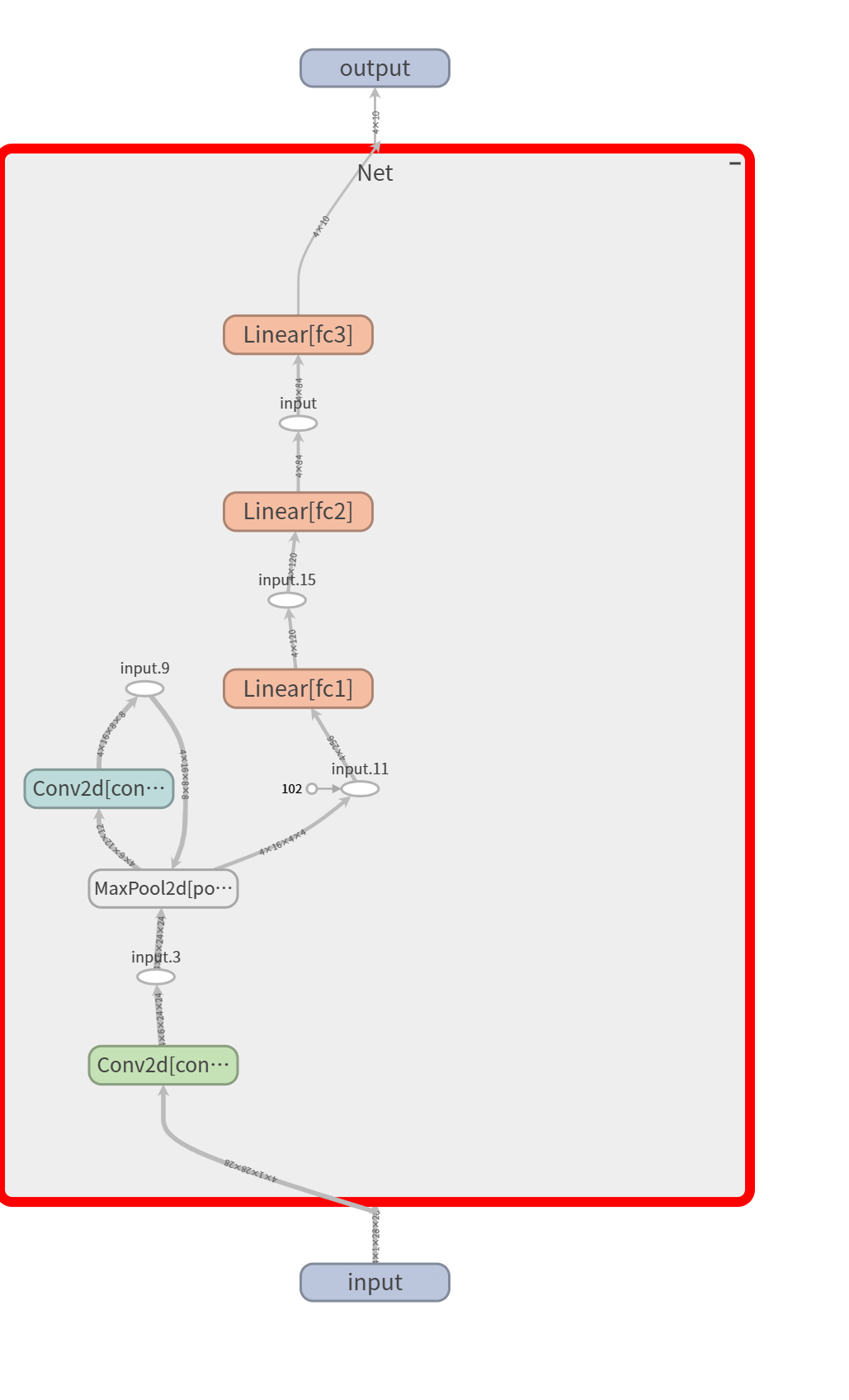

Visualizing Your Dataset

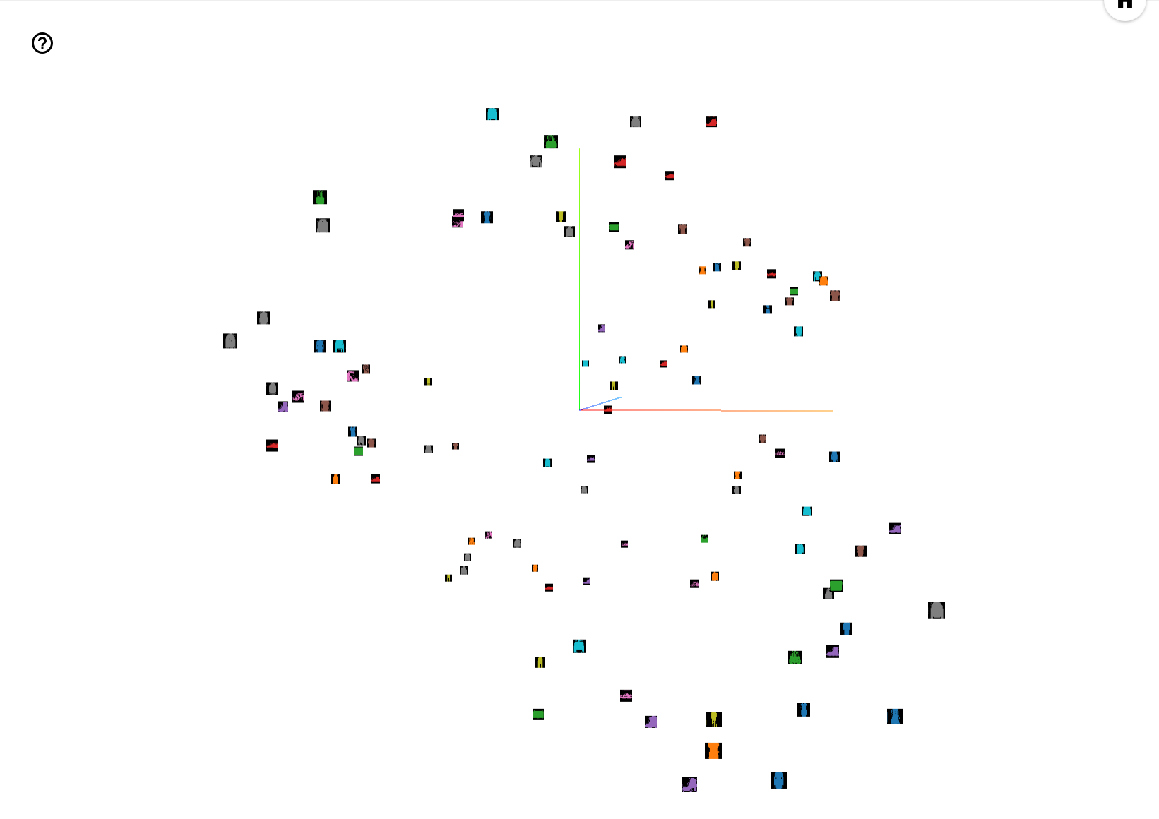
The 28-by-28 image tiles we’re using can be modeled as 784-dimensional vectors (28 * 28 = 784). It can be instructive to project this to a lower-dimensional representation. The add_embedding() method will project a set of data onto the three dimensions with highest variance, and display them as an interactive 3D chart. The add_embedding() method does this automatically by projecting to the three dimensions with highest variance.

# Select a random subset of data and corresponding labels
def select_n_random(data, labels, n=100):
    assert len(data) == len(labels)

    perm = torch.randperm(len(data))
    return data[perm][:n], labels[perm][:n]

# Extract a random subset of data
images, labels = select_n_random(training_set.data, training_set.targets)

# get the class labels for each image
class_labels = [classes[label] for label in labels]

# log embeddings
features = images.view(-1, 28 * 28)
writer.add_embedding(features,
                    metadata=class_labels,
                    label_img=images.unsqueeze(1))
writer.flush()
writer.close()