Diifusion-Conditional

这是我学习huggingface上的diffusion course时记录的一些笔记 ，希望能对你有所帮助😊

Introduction

Unconditional models don’t give much control over what is generated. We can train a conditional model that takes additional inputs to help steer the generation process, but what if we already have a trained unconditional model we’d like to use? Enter guidance, a process by which the model predictions at each step in the generation process are evaluated against some guidance function and modified such that the final generated image is more to our liking

There are a number of ways to pass in this conditioning information, such as

• Feeding it in as additional channels in the input to the UNet. This is often used when the conditioning information is the same shape as the image, such as a segmentation mask, a depth map or a blurry version of the image (in the case of a restoration/superresolution model). It does work for other types of conditioning too. For example, in the notebook, the class label is mapped to an embedding and then expanded to be the same width and height as the input image so that it can be fed in as additional channels.
• Creating an embedding and then projecting it down to a size that matches the number of channels at the output of one or more internal layers of the UNet, and then adding it to those outputs. This is how the timestep conditioning is handled, for example. The output of each Resnet block has a projected timestep embedding added to it. This is useful when you have a vector such as a CLIP image embedding as your conditioning information. A notable example is the ‘Image Variations’ version of Stable Diffusion which does exactly this.
• Adding cross-attention layers that can ‘attend’ to a sequence passed in as conditioning. This is most useful when the conditioning is in the form of some text - the text is mapped to a sequence of embeddings using a transformer model, and then cross-attention layers in the UNet are used to incorporate this information into the denoising path. We’ll see this in action in Unit 3 as we examine how Stable Diffusion handles text conditioning.

也就是我们所说的 Conditional Generation

Guidance

For example, say we wanted to bias the generated images to be a specific color. How would we go about that? Enter guidance, a technique for adding additional control to the sampling process.

Step one is to create our conditioning function: some measure (loss) which we’d like to minimize. Here’s one for the color example, which compares the pixels of an image to a target color (by default a sort of light teal) and returns the average error:

Color

def color_loss(images, target_color=(0.1, 0.9, 0.5)):
    """Given a target color (R, G, B) return a loss for how far away on average
    the images' pixels are from that color. Defaults to a light teal: (0.1, 0.9, 0.5)"""
    target = (
        torch.tensor(target_color).to(images.device) * 2 - 1
    )  # Map target color to (-1, 1)
    target = target[
        None, :, None, None
    ]  # Get shape right to work with the images (b, c, h, w)
    error = torch.abs(
        images - target
    ).mean()  # Mean absolute difference between the image pixels and the target color
    return error

Next, we’ll make a modified version of the sampling loop where, at each step, we do the following:

• Create a new version of x that has requires_grad = True
• Calculate the denoised version (x0)
• Feed the predicted x0 through our loss function
• Find the gradient of this loss function with respect to x
• Use this conditioning gradient to modify x before we step with the scheduler, hopefully pushing x in a direction that will lead to lower loss according to our guidance function

# Variant 2: setting x.requires_grad before calculating the model predictions
guidance_loss_scale = 40
x = torch.randn(4, 3, 256, 256).to(device)

for i, t in tqdm(enumerate(scheduler.timesteps)):

    # Set requires_grad before the model forward pass
    x = x.detach().requires_grad_()
    model_input = scheduler.scale_model_input(x, t)

    # predict (with grad this time)
    noise_pred = image_pipe.unet(model_input, t)["sample"]

    # Get the predicted x0:
    x0 = scheduler.step(noise_pred, t, x).pred_original_sample

    # Calculate loss
    loss = color_loss(x0) * guidance_loss_scale
    if i % 10 == 0:
        print(i, "loss:", loss.item())

    # Get gradient
    cond_grad = -torch.autograd.grad(loss, x)[0]

    # Modify x based on this gradient
    x = x.detach() + cond_grad

    # Now step with scheduler
    x = scheduler.step(noise_pred, t, x).prev_sample


grid = torchvision.utils.make_grid(x, nrow=4)
im = grid.permute(1, 2, 0).cpu().clip(-1, 1) * 0.5 + 0.5
Image.fromarray(np.array(im * 255).astype(np.uint8))

CLIP Guidance

CLIP is a model created by OpenAI that allows us to compare images to text captions. This is extremely powerful, since it allows us to quantify how well an image matches a prompt. And since the process is differentiable 可微, we can use this as a loss function to guide our diffusion model!

We won’t go too much into the details here. The basic approach is as follows:

• Embed the text prompt to get a 512-dimensional CLIP embedding of the text
• For every step in the diffusion model process:
  • Make several variants of the predicted denoised image (having multiple variations gives a cleaner loss signal)
  • For each one, embed the image with CLIP and compare this embedding with the text embedding of the prompt (using a measure called ‘Great Circle Distance Squared’)
• Calculate the gradient of this loss with respect to the current noisy x and use this gradient to modify x before updating it with the scheduler.

# @markdown load a CLIP model and define the loss function
import open_clip

clip_model, _, preprocess = open_clip.create_model_and_transforms("ViT-B-32", pretrained="openai")
clip_model.to(device)

# Transforms to resize and augment an image + normalize to match CLIP's training data
tfms = torchvision.transforms.Compose(
    [
        torchvision.transforms.RandomResizedCrop(224),  # Random CROP each time
        torchvision.transforms.RandomAffine(5),  # One possible random augmentation: skews the image
        torchvision.transforms.RandomHorizontalFlip(),  # You can add additional augmentations if you like
        torchvision.transforms.Normalize(
            mean=(0.48145466, 0.4578275, 0.40821073),
            std=(0.26862954, 0.26130258, 0.27577711),
        ),
    ]
)


# And define a loss function that takes an image, embeds it and compares with
# the text features of the prompt
def clip_loss(image, text_features):
    image_features = clip_model.encode_image(tfms(image))  # Note: applies the above transforms
    input_normed = torch.nn.functional.normalize(image_features.unsqueeze(1), dim=2)
    embed_normed = torch.nn.functional.normalize(text_features.unsqueeze(0), dim=2)
    dists = input_normed.sub(embed_normed).norm(dim=2).div(2).arcsin().pow(2).mul(2)  # Squared Great Circle Distance
    return dists.mean()
    
# ========================================

prompt = "Red Rose (still life), red flower painting"  # @param

# Explore changing this
guidance_scale = 8  # @param
n_cuts = 4  # @param

# More steps -> more time for the guidance to have an effect
scheduler.set_timesteps(50)

# We embed a prompt with CLIP as our target
text = open_clip.tokenize([prompt]).to(device)
with torch.no_grad(), torch.cuda.amp.autocast():
    text_features = clip_model.encode_text(text)


x = torch.randn(4, 3, 256, 256).to(device)  # RAM usage is high, you may want only 1 image at a time

for i, t in tqdm(enumerate(scheduler.timesteps)):

    model_input = scheduler.scale_model_input(x, t)

    # predict the noise residual
    with torch.no_grad():
        noise_pred = image_pipe.unet(model_input, t)["sample"]

    cond_grad = 0

    for cut in range(n_cuts):

        # Set requires grad on x
        x = x.detach().requires_grad_()

        # Get the predicted x0:
        x0 = scheduler.step(noise_pred, t, x).pred_original_sample

        # Calculate loss
        loss = clip_loss(x0, text_features) * guidance_scale

        # Get gradient (scale by n_cuts since we want the average)
        cond_grad -= torch.autograd.grad(loss, x)[0] / n_cuts

    if i % 25 == 0:
        print("Step:", i, ", Guidance loss:", loss.item())

    # Modify x based on this gradient
    alpha_bar = scheduler.alphas_cumprod[i]
    x = x.detach() + cond_grad * alpha_bar.sqrt()  # Note the additional scaling factor here!

    # Now step with scheduler
    x = scheduler.step(noise_pred, t, x).prev_sample


grid = torchvision.utils.make_grid(x.detach(), nrow=4)
im = grid.permute(1, 2, 0).cpu().clip(-1, 1) * 0.5 + 0.5
Image.fromarray(np.array(im * 255).astype(np.uint8))

• If you check out some code for CLIP-guided diffusion in practice, you’ll see a more complex approach with a better class for picking random cutouts from the images and lots of additional tweaks to the loss function for better performance.
• Before text-conditioned diffusion models came along, this was the best text-to-image system there was! Our little toy version here has lots of room to improve, but it captures the core idea: thanks to guidance plus the amazing capabilities of CLIP, we can add text control to an unconditional diffusion model 🎨.

Class-Conditioned DM

As mentioned in the introduction to this unit, this is just one of many ways we could add additional conditioning information to a diffusion model, and has been chosen for its relative simplicity.

Creating a Class-Conditioned UNet

The way we’ll feed in the class conditioning is as follows:

• Create a standard UNet2DModel with some additional input channels
• Map the class label to a learned vector of shape (class_emb_size)via an embedding layer
• Concatenate this information as extra channels for the internal UNet input with net_input = torch.cat((x, class_cond), 1)
• Feed this net_input (which has (class_emb_size+1) channels in total) into the UNet to get the final prediction

In this example I’ve set the class_emb_size to 4, but this is completely arbitrary and you could explore having it size 1 (to see if it still works), size 10 (to match the number of classes), or replacing the learned nn.Embedding with a simple one-hot encoding of the class label directly.

This is what the implementation looks like:

class ClassConditionedUnet(nn.Module):
    def __init__(self, num_classes=10, class_emb_size=4):
        super().__init__()

        # The embedding layer will map the class label to a vector of size class_emb_size
        self.class_emb = nn.Embedding(num_classes, class_emb_size)

        # Self.model is an unconditional UNet with extra input channels to accept the conditioning information (the class embedding)
        self.model = UNet2DModel(
            sample_size=28,  # the target image resolution
            in_channels=1 + class_emb_size,  # Additional input channels for class cond.
            out_channels=1,  # the number of output channels
            layers_per_block=2,  # how many ResNet layers to use per UNet block
            block_out_channels=(32, 64, 64),
            down_block_types=(
                "DownBlock2D",  # a regular ResNet downsampling block
                "AttnDownBlock2D",  # a ResNet downsampling block with spatial self-attention
                "AttnDownBlock2D",
            ),
            up_block_types=(
                "AttnUpBlock2D",
                "AttnUpBlock2D",  # a ResNet upsampling block with spatial self-attention
                "UpBlock2D",  # a regular ResNet upsampling block
            ),
        )

    # Our forward method now takes the class labels as an additional argument
    def forward(self, x, t, class_labels):
        # Shape of x:
        bs, ch, w, h = x.shape

        # class conditioning in right shape to add as additional input channels
        class_cond = self.class_emb(class_labels) # 得到的形状为(bs,emb_size)
        class_cond = class_cond.view(bs, class_cond.shape[1], 1, 1).expand(bs, class_cond.shape[1], w, h)
        # x is shape (bs, 1, 28, 28) and class_cond is now (bs, 4, 28, 28)

        # Net input is now x and class cond concatenated together along dimension 1
        net_input = torch.cat((x, class_cond), 1)  # (bs, 5, 28, 28)

        # Feed this to the UNet alongside the timestep and return the prediction
        return self.model(net_input, t).sample  # (bs, 1, 28, 28)

Training and Sampling

Where previously we’d do something like prediction = unet(x, t) we’ll now add the correct labels as a third argument (prediction = unet(x, t, y)) during training, and at inference we can pass whatever labels we want and if all goes well the model should generate images that match. y in this case is the labels of the MNIST digits, with values from 0 to 9.

The training loop is very similar to the example from Unit 1.

# @markdown Training loop (10 Epochs):

# Redefining the dataloader to set the batch size higher than the demo of 8
train_dataloader = DataLoader(dataset, batch_size=128, shuffle=True)

# How many runs through the data should we do?
n_epochs = 10

# Our network
net = ClassConditionedUnet().to(device)

# Our loss function
loss_fn = nn.MSELoss()

# The optimizer
opt = torch.optim.Adam(net.parameters(), lr=1e-3)

# Keeping a record of the losses for later viewing
losses = []

# The training loop
for epoch in range(n_epochs):
    for x, y in tqdm(train_dataloader):

        # Get some data and prepare the corrupted version
        x = x.to(device) * 2 - 1  # Data on the GPU (mapped to (-1, 1))
        y = y.to(device)
        noise = torch.randn_like(x)
        timesteps = torch.randint(0, 999, (x.shape[0],)).long().to(device)
        noisy_x = noise_scheduler.add_noise(x, noise, timesteps)

        # Get the model prediction
        pred = net(noisy_x, timesteps, y)  # 别的都一样，只是这里把类别值传进了unet

        # Calculate the loss
        loss = loss_fn(pred, noise)  # How close is the output to the noise

        # Backprop and update the params:
        opt.zero_grad()
        loss.backward()
        opt.step()

        # Store the loss for later
        losses.append(loss.item())

    # Print out the average of the last 100 loss values to get an idea of progress:
    avg_loss = sum(losses[-100:]) / 100
    print(f"Finished epoch {epoch}. Average of the last 100 loss values: {avg_loss:05f}")

# View the loss curve
plt.plot(losses)

Stable Diffusion 概览

In this unit you will meet a powerful diffusion model called Stable Diffusion (SD) and explore what it can do. Stable Diffusion is a powerful text-conditioned latent diffusion model.

Latent Diffusion

As image size grows, so does the computational power required to work with those images. This is especially pronounced in an operation called self-attention, where the amount of operations grows quadratically with the number of inputs. A 128px square image has 4x as many pixels as a 64px square image, and so requires 16x (i.e. 42) the memory and compute in a self-attention layer. This is a problem for anyone who’d like to generate high-resolution images!

Latent diffusion helps to mitigate this issue by using a separate model called a Variational Auto-Encoder (VAE) to compress images to a smaller spatial dimension. The rationale behind this is that images tend to contain a large amount of redundant information - given enough training data, a VAE can hopefully learn to produce a much smaller representation of an input image and then reconstruct the image based on this small latent representation with a high degree of fidelity. The VAE used in SD takes in 3-channel images and produces a 4-channel latent representation with a reduction factor of 8 for each spatial dimension. That is, a 512px square input image will be compressed down to a 4x64x64 latent.

By applying the diffusion process on these latent representations rather than on full-resolution images, we can get many of the benefits that would come from using smaller images (lower memory usage, fewer layers needed in the UNet, faster generation times…) and still decode the result back to a high-resolution image once we’re ready to view the final result. This innovation dramatically lowers the cost to train and run these models.

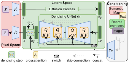
Text Conditioning

In Unit 2 we showed how feeding additional information to the UNet allows us to have some additional control over the types of images generated. We call this conditioning. Given a noisy version of an image, the model is tasked with predicting the denoised version based on additional clues such as a class label or, in the case of Stable Diffusion, a text description of the image. At inference time, we can feed in the description of an image we’d like to see and some pure noise as a starting point, and the model does its best to ‘denoise’ the random input into something that matches the caption.

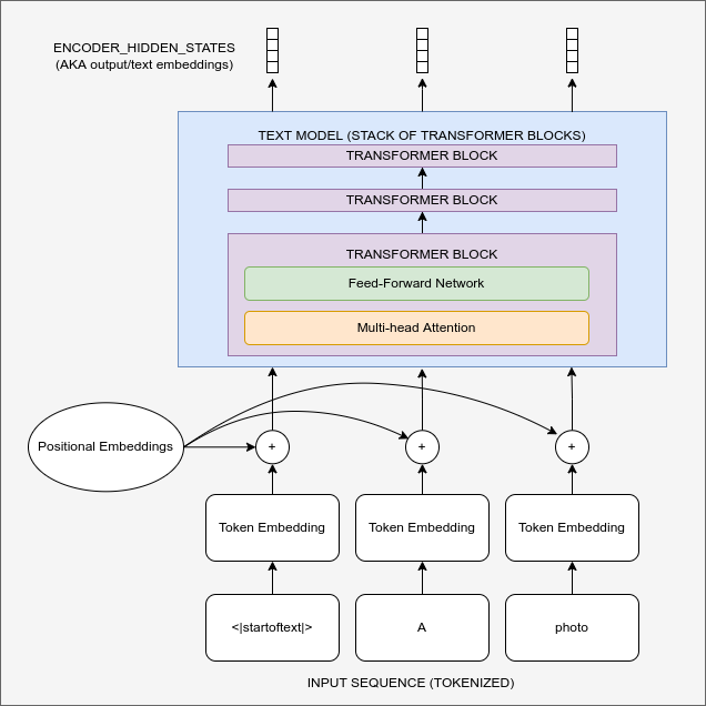
Diagram showing the text encoding process which transforms the input prompt into a set of text embeddings (the encoder_hidden_states) which can then be fed in as conditioning to the UNet.

For this to work, we need to create a numeric representation of the text that captures relevant information about what it describes. To do this, SD leverages a pre-trained transformer model based on something called CLIP.
CLIP’s text encoder was designed to process image captions into a form that could be used to compare images and text, so it is well suited to the task of creating useful representations from image descriptions. An input prompt is first tokenized (based on a large vocabulary where each word or sub-word is assigned a specific token) and then fed through the CLIP text encoder, producing a 768-dimensional (in the case of SD 1.X) or 1024-dimensional (SD 2.X) vector for each token. To keep things consistent prompts are always padded/truncated to be 77 tokens long, and so the final representation which we use as conditioning is a tensor of shape 77x1024 per prompt.

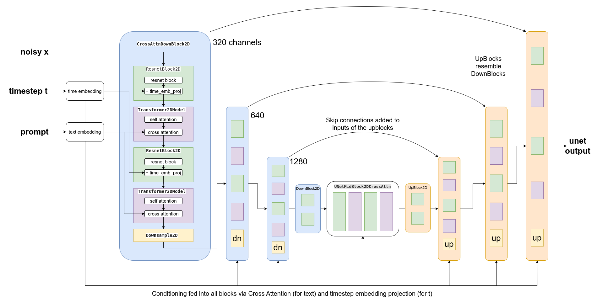
OK, so how do we actually feed this conditioning information into the UNet for it to use as it makes predictions? The answer is something called ==cross-attention==. Scattered throughout the UNet are cross-attention layers. Each spatial location in the UNet can ‘attend’ to different tokens in the text conditioning, bringing in relevant information from the prompt. The diagram above shows how this text conditioning (as well as timestep-based conditioning) is fed in at different points. As you can see, at every level the UNet has ample opportunity to make use of this conditioning!

Classifier-free Guidance

研究发现，即便我们竭尽全力优化文本条件的效果，模型在预测时仍倾向于主要依赖含噪输入图像而非提示词。某种程度上这可以理解——许多图像说明文字与其对应图片关联性较弱，因此模型学会了不过度依赖文字描述！但在生成新图像时，这种行为就不可取了——如果模型不遵循提示词，我们可能得到与描述完全无关的图像。

To fix this, we use a trick called Classifier-Free Guidance (CGF). During training, text conditioning is sometimes kept blank, forcing the model to learn to denoise images with no text information whatsoever (unconditional generation). Then at inference time, we make two separate predictions: one with the text prompt as conditioning and one without. We can then use the difference between these two predictions to create a final combined prediction that pushes even further in the direction indicated by the text-conditioned prediction according to some scaling factor (the guidance scale), hopefully resulting in an image that better matches the prompt. The image above shows the outputs for a prompt at different guidance scales - as you can see, higher values result in images that better match the description.

• 类似 dropout ,然后通过一个系数来控制guidance的强度